Gene Expression Pattern Preprocessing
-- Manual --
Javier Herrero
Bioinformatics Unit. CNIO
3rd October 2002
Gene expression data are ratios of expression levels of two different
samples. Usually, one sample corresponds to the experimental condition
and the other one is a reference sample (Figure 1).
Figure 1:
Experimental design
|
| mRNA is extracted from two different samples and labeled with a fluorescent
probe. Both samples are mixed before hybridization. |
|
A gene expression pattern is a suite of expression data for a gene
along a suite of different experimental conditions (Figure 2).
Figure 2:
Different representations
of two gene expression patterns
|
| (A) Gene expression patterns in a common plot. (B)
Gene expression patterns in a color scale. In this case, higher values
appear in green and lower ones in red. |
|
Since we are looking at expression ratios, we will get the patterns
in an asymmetrical scale: over-expressions will have values between
1 and infinite while over-repressions will be between 1 and 0. In
order to give the same weight to both over-expressions and over-repressions
we need to transform the scale (Figure 3).
The most common function used for this task is the log-transformation.
Figure 3:
Log-Transformation
|
| (A) Gene expression patterns before log-transformation: gene
B seems to be nearly flat (B) Gene expression patterns after
log-transformation: it is now possible to see that gene A and gene
B are symmetrical. |
|
The Expression Data Preprocessor has a function for log-transforming
the patterns (Figure 4). You can choose
among 2, e and 10 for the base of log-transformation.
Figure 4:
Interface to log-transformation
function
|
|
In order to check the quality of the final result it is usual to spot
several times the same cDNA clone or different ones representing the
same gene on the cDNA array. We will get several values of expression
for those genes but we would like to have only one to continue the
analysis of the results.
The solution is quite simple: we have to get the average or the median
value of all the replicates, but it is desirable to check first on
inconsistencies among replicates. The system includes a function for
removing inconsistent replicates based on maximum distance to median.
For each replicated gene, it calculates the median and remove all
the values that are beyond the threshold from the median (Table 1).
Table 1:
Examples of inconsistent
replicate removing
| |
Replicated values |
Median |
Threshold |
Accepted range |
Resulting values |
| 1 |
2.6; 3.8 |
3.2 |
1.0 |
2.2 -- 4.2 |
2.6; 3.8 |
| 2 |
1.3; 1.6; 3.8 |
1.6 |
1.5 |
0.1 -- 3.1 |
1.3; 1.6 |
| 3 |
-2.2; -1.8; -1.6; 0.3 |
-1.7 |
1.0 |
-2.7 -- -0.7 |
-2.2; -1.8; -1.6 |
| 4 |
0.8; 4.2 |
2.5 |
1.0 |
1.5 -- 3.5 |
-- |
| 5 |
-0.3; 1.1; 1.3 |
1.1 |
0.5 |
0.6 -- 1.6 |
1.1; 1.3 |
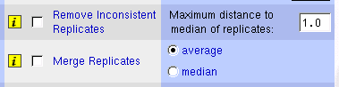
Once inconsistent replicates have been removed, it is possible to
merge them together. Two options are available at this stage: getting
the average or the median of the replicates (Table 2).
Table 2:
Examples of replicate merging
| |
Resulting values |
Average |
Median |
| 1 |
2.6; 3.8 |
3.2 |
3.2 |
| 2 |
1.3; 1.6 |
1.45 |
1.45 |
| 3 |
-2.2; -1.8; -1.6 |
-1.87 |
-1.8 |
| 5 |
1.1; 1.3; 1.8 |
1.4 |
1.3 |
Figure 5:
Interface to replicate handling
functions
|
|
One of the characteristic of the gene expression patterns is the existence
of missing values in the data set. The excess of missing values can
be a problem for standard hierarchical clustering methods where all
the calculations are based on a distance matrix. If two patterns have
not enough points in common, the distance between them will be undefined
and the clustering will fail. Moreover, other methods like principal
component analysis cannot deal with missing values. Using imputation
for these values can bypass these problems but it could be still necessary
to remove beforehand some patterns if there are not enough data (see
[Troyanskaya et al., 2001] for further reading).
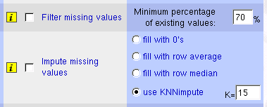
The function for removing patterns with too many missing values is
based on the percentage of existing values, i.e., on the percentage
of non-missing values (Table 3)
Table 3:
Examples of removing patterns
with excess of missing values
| |
Length of patterns
(number of conditions)
|
|
|
Number of
existing values
|
|
Persentage of
existing values
|
|
Result |
| 1 |
10 |
3 |
7 |
70 % |
Accept |
| 2 |
20 |
7 |
13 |
70 % |
Remove |
| 3 |
5 |
3 |
2 |
50 % |
Remove |
| 4 |
12 |
2 |
10 |
75 % |
Accept |
Actually, the system has 4 different options for imputing missing
values: (1) filling blanks with zeros, (2) with row (pattern) average,
(3) with row median or (4) using KNN-imputation method. KNN-imputation
method is a method which uses the K nearest neighbors (where
K is a user-defined parameter and euclidean distance is used
for determining the nearest neighbors) to impute the missing values
(Table 4).
In principle KNN-imputation works much better than the other methods
but it requires to have enough complete patterns (patterns with no
missing values) in the data set to be confident of finding real neighbors
of the patterns with missing values. It also requires to have enough
existing values in patterns with missing values in order to be able
to determine their neighbors. Usually one expect to have at least
1000 complete patterns in the data set and at the very minimum 5 existing
values for using this method.
Figure 6:
Interface to missing value
handling functions
|
|
It is desirable to remove flat patterns because we cannot distinguish
signal form noise in such patterns. Moreover, we will get strange
results while clustering if we use a correlation metrics since flat
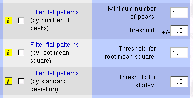
patterns can correlate with nearly anything. There are different functions
for flat patterns filtering depending on the actual definition of
``flat'' pattern. The simplest one is based on number of peaks
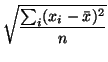
in the pattern. The other two functions are based on the variability
of the values in the pattern: the root mean square (RMS; cf. (1))
and the standard deviation (stddev; cf. (2)).
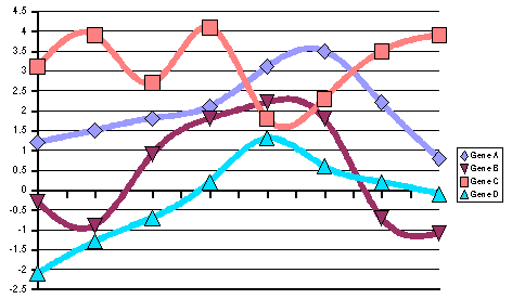
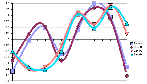
In those examples (Figure 7) we see
the difference between RMS and stddev: genes A and C have an RMS much
higher than their stddev because the average value of their patterns
is far from zero, whereas genes B and D show nearly the same RMS as
stddev because their average values are approximately zero.
Different authors used different methods. For example, [Iyer et al., 1999]
used a combination of peak and stddev for filtering flat patterns:
they only took into account patterns (in  scale) with at
least two peaks greater than 2.2 (or lower than -2.2) and patterns
with a stddev greater than 0.7. [Chu et al., 1998] used
a threshold of 1.13 of RMS (in scale) for filtering flat
patterns.
scale) with at
least two peaks greater than 2.2 (or lower than -2.2) and patterns
with a stddev greater than 0.7. [Chu et al., 1998] used
a threshold of 1.13 of RMS (in scale) for filtering flat
patterns.
Figure 8:
Interface to flat pattern
filtering functions
|
|
All previous filters were based on the gene expression patterns, whereas
this one is based on the names of the genes. The Expression
Data Preprocessor reads a list of known genes from an extra file
and removes all the patterns corresponding to genes that are not present
in this list. This option can be used if you want to concentrate in
a particular family of genes, or apply the filtering steps from a
different dataset. For example, it is possible to apply several filtering
criteria to a subset of the experimental conditions and use the result
to filter the original dataset.
Figure 9:
Interface to unknown gene
removing function
|
|
Finally, there is an option for standardizing the patterns. Pattern
standardization is nothing but subtracting the average value of the
pattern to each value and dividing the result by the stddev (cf. (![[*]](crossref.png) )):
)):
Figure 11:
Examples of gene expression
patterns after standardization
|
B
| |
x |
x |
x |
x |
x |
x |
x |
x |
Average |
stddev |
| A |
1.20 |
2.60 |
3.20 |
2.00 |
3.10 |
4.30 |
3.70 |
1.40 |
2.69 |
1.10 |
|---|
| B |
-0.50 |
0.20 |
0.40 |
-0.50 |
0.40 |
0.90 |
0.60 |
-0.90 |
0.08 |
0.63 |
|---|
| C |
-2.50 |
-3.20 |
-3.10 |
-2.20 |
-0.80 |
-1.30 |
-0.50 |
-1.70 |
-1.91 |
1.01 |
|---|
| D |
1.50 |
0.80 |
0.70 |
1.50 |
3.10 |
2.50 |
3.40 |
2.70 |
2.03 |
1.04 |
|---|
| (A) Representation of expression patterns of genes A, B,
C and D before pattern standardization. (B) Numerical values
of their expression patterns, their average value and their stddev. |
Figure 10:
Examples of gene expression
patterns before standardization
|
 |
B
| |
x |
x |
x |
x |
x |
x |
x |
x |
Average |
stddev |
| A |
1.36 |
-0.08 |
0.47 |
-0.63 |
0.38 |
1.47 |
0.92 |
-1.17 |
0.0 |
1.0 |
|---|
| B |
-0.91 |
0.20 |
0.51 |
-0.91 |
0.51 |
1.31 |
0.83 |
-1.54 |
0.0 |
1.0 |
|---|
| C |
-0.58 |
-1.27 |
-1.18 |
-0.28 |
1.10 |
0.61 |
1.40 |
0.21 |
0.0 |
1.0 |
|---|
| D |
-0.51 |
-1.18 |
-1.28 |
-0.51 |
1.04 |
0.46 |
1.33 |
0.65 |
0.0 |
1.0 |
|---|
| (A) Representation of expression patterns of genes A, B,
C and D after pattern standardization. (B) Numerical values
of their expression patterns, their average value and their stddev. |
|
This function is used to bring all the patterns of the data set into
the same range for an easier comparison. In particular, this transformation
is applied when one wants to calculate correlations among gene expression
patterns but the method he wants to use only permits to calculate
euclidean distances: an euclidean metrics to standardized patterns
is comparable to a correlation metrics on original patterns.
Nevertheless, pattern standardization present a serious drawback when
dealing with flat patterns: the method can produce a big noise if
the stddev of the pattern is close to zero, moreover, the result is
undefined if the stddev is exactly zero. Thus it is desirable to remove
flat patterns beforehand.
Figure 12:
Interface to pattern standardization
function
|
|
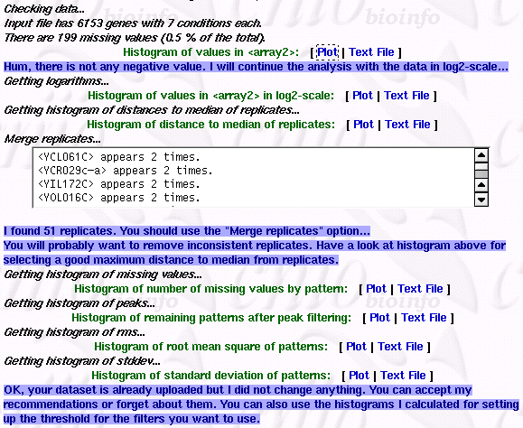
The most interesting feature of this interface is its Pre-Analysis
module. It performs several checks and plots different histograms
to help and to guide the user through the options. It automatically
selects or unselects different options and gives useful information
to the user.
Here is the list of topics covered by the pre-analyse module:
- File format: it checks that all the patterns have the
same number of conditions. It adds extra missing values or removes
extra ones if needed. It also checks that all the patterns have a
valid identifier. It adds a unique one when necessary. It also keeps
a list of symbols interpreted as missing values and displays
this information. A warning message is displayed if there are too
many of them, as could happen if the file uploaded is in a wrong format.
- Dimensions of the data set: the server expects a dataset
with more rows (genes) than columns (experimental conditions). It
displays a warning message if it founds more conditions than patterns,
as could happen if the data matrix is transposed.
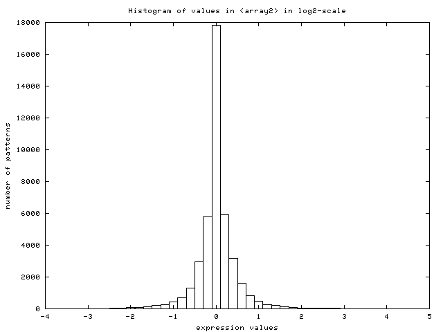
- Scale of expression patterns: the server plots the histogram
of values found in the data set (Figure 14) and
looks for negative values. It assumes the user did not log-transform
the dataset if none is found. It displays a warning message, log-transforms
the data internally to continue with the analysis, auto-selects the
option for log-transforming the dataset and plots the new histogram
of log-transformed values (Figure 15).
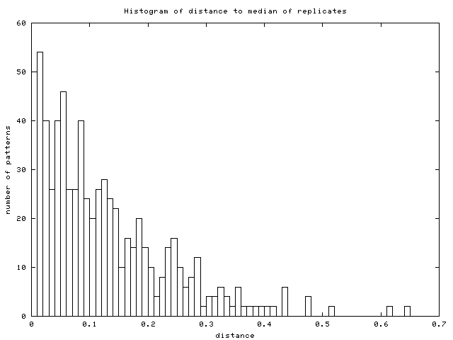
- Replicated genes: the server looks for replicated genes and
merge them into their average pattern. The list of replicated genes
as well as the number of them is displayed. The server also plots
an additional histogram of distances to median of replicates (Figure
16) to guide user in selecting a good threshold
for removing inconsistent replicates.
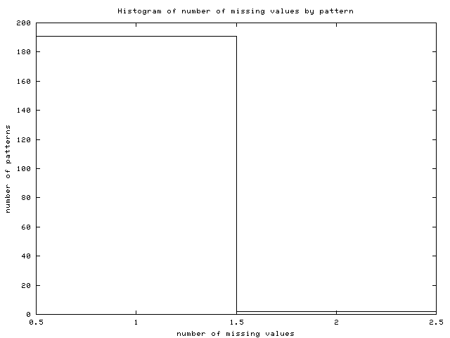
- Missing values: the server obtains the number of missing
values for this dataset and suggests the best imputation method among
the available ones depending on the amount of missing values, the
amount of complete patterns and the number of conditions. It also
plots an histogram of the number of missing values by pattern (Figure
17).
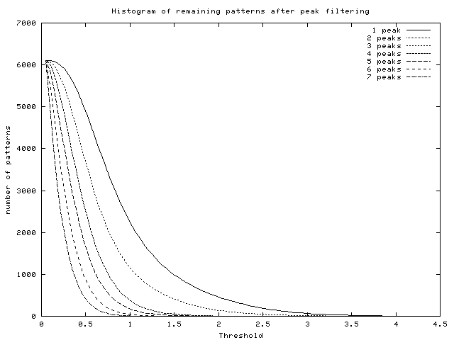
- Histogram of peaks: this histogram informs the user about
the number of remaining profiles after using the ``Filter flat
patterns by number of peaks'' option versus the threshold used (see
Figure 18).
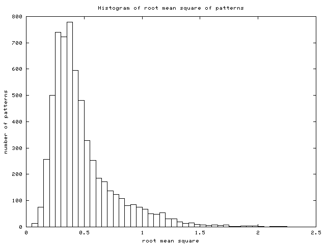
- Histogram of RMS: this is the histogram of RMS in the data
set (see Figure 19).
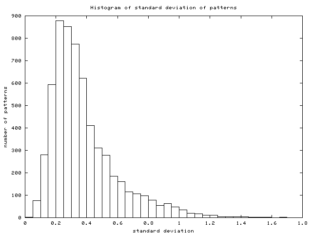
- Histogram of stddev: this is the histogram of stddev in the
data set (see Figure 20).
It is important to emphasize that the Pre-Analyse module does not
change the original file: the user can ignore the recommendations
simply by unselecting the corresponding options.
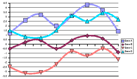
Figure 15:
Histogram of values in the data set
after log2-transformation (data from [DeRisi et al., 1997])
|
|
Figure 16:
Histogram of distances from replicates
to their median (data from [DeRisi et al., 1997])
|
|
Figure 18:
Histogram of remaining patterns after
peak filtering (data from [DeRisi et al., 1997])
|
|
All functions have a small square with an ``i'' inside: this is
a link to the help section related to that function (see Figures 4,
5, 6, 8,
9 and 12).
If your browser understands and uses JavaScript, you can click on
the names of the functions for setting and unsetting them (see Figures
4, 5, 6,
8, 9 and 12)
and on the names of their options (see Figures 5
and 6) for selecting them.
This server returns four kinds of messages:
- Useful Information is displayed in black.
- Output from some functions will appear in scrollable text
boxes.
- Harmless warning messages are written in blue.
- More serious warning messages appear in red.
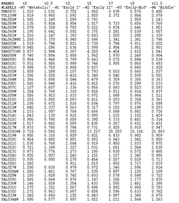
- This server uses plain text file as input. The gene expression patterns
must appear in a table separated by tabulators where each line
corresponds to a gene and each column to an experimental condition.
The first column must contain the gene names.
- There is no special character for missing values, simply leave
these places empty.
- All lines beginning with a ``#'' are ignored.
- This server does not need to know the name of the conditions,
but you can specify them by adding a row to the table where the first
element must be ``#NAMES''.
- You can add class labels to the genes by appending an ``@''
and a number to the name of the gene. You can also set up the names
of those class labels by adding a line starting by ``#LABELS''
(see Figure 21 for an example).
Preprocessed data will appear in the same format as the input file
format. The file contains a comment line for each function used. This
is the file format understood by the hierarchical clustering and the
SOTA [Herrero et al., 2001] servers. Additionnaly, there is
an extra file for SOM [Kohonen, 1997] and SomTree [Herrero & Dopazo, 2002],
two files for sending the preprocessed data set to the EPClust [Brazma & Vilo, 2000]
and a file containing the list of removed genes. The last one is used
in the FatiGO (Al-Shahrour et al., in preparation) analysis
for comparing removed against remaining genes.
In SOM file format the gene names appear at the end of the patterns
and the first line must contain the length of patterns. EPClust is
able to use two different file: one for gene expression patterns and
the other one for gene descriptions.
Uploaded data set are saved in temporary directories in the server and are
accessible through the web until they are erased after some time. Anybody can
access those directories, nevertheless the name of the directories are not
trivial, thus it is not easy for a third person to access your data.
In any case, you should keep in mind that communications between the client
(your computer) and the server are not encripted at all, thus it is also
possible for somebody else to look at your data while you are uploading or
dowloading them.
All the data set needed for these exercises are available
here
- Go to the ``Diauxic Shift'' [DeRisi et al., 1997]
data set web page
[Click here]
- Send the data set to the Preprocessor by clicking on ``preprocess''
- Pre-Analyse the data set by clicking on the ``Pre-Analyse'' button.
- How many gene expression patterns are in the data set?
- How many of them are replicated?
- Are there a lot of missing values?
- Was the data set already in a symmetrical scale?
- How many gene expression patterns have 3 missing values?
- How many genes will remain if we want to keep only genes with at least
3 peaks higher than 1 or lower than -1 (in a scale)
- Which functions are activated by default?
- Go to the ``Yeast cell cycle'' [Spellman et al., 1998]
data set web page
[Click here]
- Send the data set to the Preprocessor by clicking on ``preprocess''
- Pre-Analyse the data set by clicking on the ``Pre-Analyse'' button.
- How many gene expression patterns are in the data set?
- Was the data set already in a symmetrical scale?
- How many of them are replicated?
- Are there a lot of missing values?
- How many gene expression patterns have no missing values?
- Which method will you use if you want to impute missing values?
- How many genes will be removed if we use the ``Filter flat patterns
by RMS'' option with a threshold of 2 (in a scale)?
- And if we use a threshold of 0.2 (in a scale)?
- Which functions are activated by default?
- Go to the ``Response of Human Fibroblasts to Serum'' [Iyer et al., 1999]
data set web page
[Click here]
- Send the data set to the Preprocessor by clicking on ``preprocess''
- Pre-Analyse the data set by clicking on the ``Pre-Analyse'' button.
- How many gene expression patterns are in the data set?
- Was the data set already in a symmetrical scale?
- How many missing values are in the data set?
- Propose a good threshold of maximum distance to median of replicates
for removing inconsistent replicates.
- Are the patterns already standardized?
- Which functions are activated by default?
- Activate the ``Remove Inconsistent Replicates'' function and put
the threshold you proposed before.
- Activate and set up any combination of flat pattern filtering function.
- Click on the ``Run'' button.
- How many gene expression patterns are now in the data set?
- Is the data set in a symmetrical scale?
- How many files do appear?
- What are the differences between <fibroblasts_ori.txt> and <fibroblasts_ori.dat>?
- Go to the ``Lymphoma/leukemia Molecular Profiling Project'' [Alizadeh et al., 2000]
data set web page
[Click here]
- Send the data set to the Preprocessor by clicking on ``preprocess''
- Pre-Analyse the data set by clicking on the ``Pre-Analyse'' button.
- Is the data set already in a symmetrical scale?
- How many missing values are in the data set?
- How many complete gene expression patterns are available for KNN imputation?
- Activate the ``Log-transform'' function and choose your preferred
base for logarithm.
- Activate the ``Impute missing values'' function and choose the
``use KNNimpute'' option.
- Activate the ``Filter flat patterns by standard deviation'' function
and set up the threshold to 3.
- Click on the ``Run'' button.
- What happen when the server tried to log-transform the data set?
- How many complete gene expression patterns are available for KNN imputation
now? Why?
- How many gene expression patterns are now in the data set?
- Alizadeh et al., 2000
-
Alizadeh, A. A., Eisen, M. B., Davis, R. E., Ma, C., Lossos, I. S., Rosenwald,
A., Boldrick, J. C., Sabet, H., Tran, T., Yu, X., Powell, J. I., Yang, L.,
Marti, G. E., Moore, T., Jr, J. H., Lu, L., Lewis, D. B., Tibshirani, R.,
Sherlock, G., Chan, W. C., Greiner, T. C., Weisenburger, D. D., Armitage,
J. O., Warnke, R., Levy, R., Wilson, W., Grever, M. R., Byrd, J. C.,
Botstein, D., Brown, P. O. & Staudt, L. M. (2000).
Distinct types of diffuse large B-cell lymphoma identified by gene
expression profiling.
Nature, 403:503-511.
- Brazma & Vilo, 2000
-
Brazma, A. & Vilo, J. (2000).
Gene expression data analysis.
FEBS Letters, 480(1):17-24.
- Chu et al., 1998
-
Chu, S., DeRisi, J., Eisen, M., Mulholland, J., Botstein, D., Brown, P. O. &
Herskowitz, I. (1998).
The Transcriptional Program of Sporulation in Budding Yeast.
Science, 282(5389):699-705.
- DeRisi et al., 1997
-
DeRisi, J. L., Iyer, V. R. & Brown, P. O. (1997).
Exploring the metabolic and genomic control of gene expression on a
genomic scale.
Science, 278:680-686.
- Herrero & Dopazo, 2002
-
Herrero, J. & Dopazo, J. (2002).
Combining hierarchical clustering and self-organizing maps for
exploratory analysis of gene expression patterns.
Journal of Proteome Research, 1(5):467-470.
- Herrero et al., 2001
-
Herrero, J., Valencia, A. & Dopazo, J. (2001).
A hierarchical unsupervised growing neural network for clustering
gene expression patterns.
Bioinformatics, 17(2):126-138.
- Iyer et al., 1999
-
Iyer, V. R., Eisen, M. B., Ross, D. T., Schuler, G., Moore, T., Lee, J. C. F.,
Trent, J. M., Staudt, L. M., Jr., J. H., Boguski, M. S., Lashkari, D.,
Shalon, D., Botstein, D. & Brown, P. O. (1999).
The transcriptional program in the response of human fibroblasts to
serum.
Science, 283:83-87.
- Kohonen, 1997
-
Kohonen, T. (1997).
Self-organazing Maps.
Springer-Verlag, Berlin.
- Spellman et al., 1998
-
Spellman, P. T., Sherlock, G., Zhang, M. Q., Iyer, V. R., Anders, K., Eisen,
M. B., Brown, P. O., Botstein, D. & Futcher, B. (1998).
Comprehensive Identification of Cell Cycle-regulated Genes of the
Yeast Saccharomyces cerevisiae by Microarray Hybridization.
Mol. Biol. Cell, 9(12):3273-3297.
- Troyanskaya et al., 2001
-
Troyanskaya, O., Cantor, M., Sherlock, G., Brown, P., Hastie, T., Tibshirani,
R., Botstein, D. & Altman, R. B. (2001).
Missing value estimation methods for DNA microarrays.
Bioinformatics, 17(6):520-525.