Tutorials

1.1. cDNA arrays

Gene expression data are ratios of expression levels of two different samples. Usually, one sample corresponds to the experimental condition and the other one is a reference sample (Figure 1.1.1).



	Fig. 1.1.1   mRNA is extracted from two different samples and labeled with a fluorescent probe. Both samples are mixed before hybridization.


Both pools of laballed mRNA are mixed and hybridized to the array. Depending on the relative amount of mRNA for a specific gene in the original samples, there will be more mRNA coming from one sample or the other one hybridized to the corresponding spot (Figure 1.1.2).



	A		B
	Fig. 1.1.2   (A) Spot before hybridisation: The cDNA's are spotted on the slide.   (B) Spot after hybridisation: The labelled mRNA's are hybridized to the cDNA. The relative amount of the fluorescent probes depend relative amount of mRNA in the original samples,.

1.2. Gene expression patterns

A gene expression pattern is a suite of expression data for a gene along a suite of different experimental conditions (Figure 1.2.1).

	A
	B
	Fig. 1.2.1   Different representation of gene expression patterns   (A) Normal plot   (B) Gene expression pattern in a colorscale.

1.3. Scale Transformation

Since we are looking at expression ratios, we will get the patterns in an asymmetrical scale: over-expressions will have values between 1 and infinite while over-repressions will be between 1 and 0. In order to give the same weight to both over-expressions and over-repressions we need to transform the scale (Figure 1.3.1). The most common function used for this task is the log-transformation.

	A
	B
	Fig. 1.3.1   Gene expression pattern:   (A) Gene expression patterns before log-transformation: gene B seems to be nearly flat.   (B) Gene expression patterns after log-transformation: it is now possible to see that gene A and gene B are symmetrical.

1.4. Distance functions

Depending on what are you looking for, you can use a given distance function. There are two main families of distances:
• euclidean, that depend on the point to point differences and accounts for absolute differences
• correlation that accounts for trends.
The picture shows the different results we can obtain using the different types of distances. Using an euclidean distance, blue and red patterns will be clustered with preference to the green one, on the basis of their lower absolute differences. Using a correlation, blue and green patterns will be preferentially clustered because of their similar trends. Usually correlation has more biological meaning.

	Fig. 1.4.1   This picture shows the different results we can obtain using the different types of distances. Using an euclidean distance, blue and red patterns will be clustered with preference to the green one, on the basis of their lower absolute differences. Using a correlation, blue and green patterns will be preferentially clustered because of their similar trends.


Usually correlation has more biological meaning.

1.5. Clustering with UPGMA

The UPGMA is an aglomerative hierarchical method. It starts by calculating the all-to-all distance matrix. The two closest patterns are merged and the all-to-all disance matrix is calculated again but using the new cluster instead of the two merged patterns. This process is repeated until the complete dendrogram is built.

	A
	B
	C
	D
	Fig. 1.5.1   UPGMA: the all-to-all distance matrix (black box) is calculated and two closest elements (red box) are merged.   (A) The two closest elements are genes B and C.   (B) The genes B and C are merged and the all-to-all distance matrix is calculated again using the new cluster instead of the genes B and C. Now, the two closest elements are genes A and D.   (C) The genes A and D are also merged. The elements must be reordered to fit the topology of the tree. The all-to-all distance matrix is calculated again with the two remaining elements.   (D) The process ends when all the complete dendogram is built.

1.6. Clustering with SOM

SOM is Neural Network based on a lattice of nodes or neurons. Usual lattices are rectangular or hexagonal. The nodes have an associated vector of the same length of the input data. At the beginning, all nodes have random values and the training starts. The first item is compared with all the nodes of the lattice to get the closest node. This node is called the winning node and itself and its neighbourhood are updated, i.e., they are changed to make it closer to the item. The strength of the updating of a node depends on the distance of this node to the winning node. A cycle ends when this process has been performed for all the input items. The training ends when a predefined number of cycles has been performed.

Available parameters include the number of repetitions (the training length), the strength of the updating (the training rate) and the size of the neighbourhood (the radius). Usually the training is performed in two phases: the first one is the ordering phase (strong training rate and large radius) and the last one is the fine-tunning phase (long training with a weak training rate and a smaller radius)



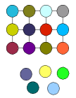
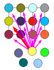
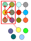
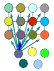
A			B			C		D
Fig. 1.6.1   Schematic representation of the working of SOM network   (A) The lattice has random values at the beginning.   (B) The first element is compared with all the nodes of the lattice to get the closest node (red arrow).   (C) The winning node and its neighbourhood are updated.   (D) Next item is compared with all the nodes of the lattice as in (B). This process is repeated thousands of times for all the items. .

1.7. Clustering with SOM-Tree

This approach combines both Hierarchical Clustering and SOM. First the size of the problem is reduced with SOM. A flat network is obtained where each node has an associated vector representing the average pattern of expression of the genes that fall into that node. Then Hierarchical Clustering is used to group those clusters. At the end a hierarchical tree is obtained where the leaves correspond the original nodes coming from the SOM and the branch lengths are proportional to the distances among the nodes, which represent groups of co-expressing genes.

1.8. Clustering with SOTA

SOTA is a divisive method, that starts the classification with a binary topology compose of a root node with two leaves. The self-organizing process splits the data (e.g. experimental gene profiles) into two clusters (see Fig 1.8.1). After reaching convergence at this level, the network is inspected. If the level of variability in one, or more, terminal nodes is over a given threshold, then, the tree grows by expanding these terminal nodes. Two new descendants are generated from this heterogeneous node that becomes internal and does not receive direct updates from the data in future steps. The growth of the network is directed by the resource value that is defined as the mean value of the distances between a node and the expression profiles associated with it (Dopazo and Carazo, 1997; Fritzke, 1994).


A			B
			C
			D
			E
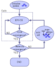
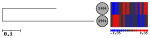
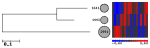
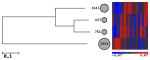
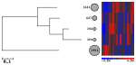
Fig. 1.8.1   (A) Schematic representation of the growing algorithm of SOTA network   The neurons that compose the network are represented as vectors (rows of the data matrix) whose components correspond to the columns of the data matrix, that is, to the experiments at which each gene expression values have been measured. On the top, the Initial state of the network, with two terminal neurons, called cells, connected by an internal neuron called node. Cycle: repeat as many epochs as necessary to reach convergence (the error falls below a given threshold) in the present topology of the network. When a cycle finishes, the network size increases: two new neurons are attached to the neuron with higher resources. This neuron becomes mother neuron and does not receive direct inputs any more. Once the variability of all the neurons is below a given threshold the network growing ends.   (B), (C), (D) and (E) Step-by-step growing of SOTA: the size of circles represents the amount of gene in the cluster and pattern of the cluster is drawn in a colorscale from blue to red.


SOTA structures grow from the root of the tree, toward the leaves, producing a representation of the data from lower to higher resolution. If the growth of the network is not restricted, the outcome would be a binary tree which contains only one profile in each leave. Nevertheless, if a threshold of resource value has been fixed, once all terminal nodes fall below such a threshold, the expansion of the binary topology will be stopped. This allows the generation of a hierarchical cluster structure at the desired level of resolution (see Herrero et al., 2001 for details)