24444 entries updated 24th
February 2004  http://www.rcsb.org/pdb |
22,318,883 in year 2002
(February 2003)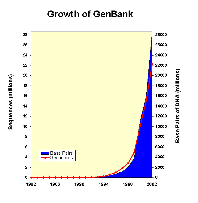 http://www.ncbi.nlm.nih.gov/Genbank/genbankstats.html |
This sections aims to deal with all the theoretical an practical course of 1D predicitions.
| PROTEIN 1D PREDICTIONS | [BACK TO MAIN] |
There are not
methods available to predict the protein 3D structure (folding) from
the amino acid sequence. However, there are well established methods
allowing to predict more simple structural features. These features can
provide with useful indormation.
Due to the
genome sequencing projects the number of sequences has increased
exponentially. Nonetheless, the crystal structures are not growing at
the same rate (see figures below in the table). Then we have about
25.000 crystal structures (year 2004) whereas at the same time there
are about 22 millions (year 2002). Why such a shift?
Technically, is easier to obtain a DNA sequence (and then translate it)
than obtaining a X-ray or NMR structure. We can obtain a DNA sequence
in 2-3 days whereas the experimental requirements to obtain crystal
might varie between 1-3 years.
24444 entries updated 24th
February 2004
http://www.rcsb.org/pdb 22,318,883 in year 2002
(February 2003)
http://www.ncbi.nlm.nih.gov/Genbank/genbankstats.html
It has been proposed (and most of the times proven) that the protein 3D
structure is a consequence of its primary amino acid composition.
However there are many other factors that could influence the folding of
a given protein. For instance chaperone proteins are essential for
folding. But generally speaking it is assumed that the final structure
is represented by the form in its minimum free energy state. That's why
the native structure is coded by its primary amino acid sequence.
There are some limits to this assumption. For example, there is not
accuracy to establish the basic parameters improtant for folding, and
also the computing resources are not well developed in these terms so
far. There is not possible to predict structure from primary sequence
yet as inferred by CASP experiments.
We can, however, assign secondary structure elements
to a primary sequence. In a 3 state condition, there are several
algorithms capable to conduct such assignations. This can be useful for
further attempts to thread. In fact, the most advanced methods are
those regarding predicting secondary structure. This has happened
because of the combiantion of such methods and evolutionary information
available in the databases.
The 1D structural predictions even if partially wrong, are very useful to obtain information regarding function of a given protein. Sometimes we can extract information related to the active site of a protein and even perform more complex predictions
Residue properties
The primary data we can extract from a protein are its physico-chemical characteristics like:
hydrophobicity, polarity, etc. ExPASy Tools: ProtScale
(hidrophobicity among others, amino acid level)
This server inputs a query and allows to select within 54 parameters. Biological software, Institute
Pasteur: Protein
Properties(hidrophobicity among others, amino acid level)>
2.- Another way to describe the methods are based on the algorithm: First generation methods:
Statistical methods analzying amino acid propensity to adopt certain secondary structures.
The firt one (Chou & Fasman, 1975). Inference of data coming from 15 X-ray structures.
The reliability for this method is ~ 50% (when 62 proteins are used to infer statistics) Second generation methods
The main improvement relies on the combination of using the major databases and calculating statistics based on neighbour segments (11-21 residues).
The statistics evaluates the propensity of the central residue to be in a given secondary structure.
First and second generation methods show obvious problems
Reliability (3 state predictions) <70% Reliability for B-strands 28-48% (~random) alpha and beta too short This is due to: Experimental structures vary even within crystals of the same protein Secondary structure depends on long range interactions (more than 11-21 resideues). This effect is stronger for betas.
. Third generation methods The inclusion of evolutionary information allowed to improve the reliability of the predictions.The profiles obtained from multiple alignments are indicative of structural constrains. Moreover, these profiles don't contain local information as the evolutive preassure takes place at the 3D level and not at the priamry sequence level.
Therefore PSI-BLAST and Hidden Markov models improve remarkably the predictions.
Pros: relaibility (3-state predictions) 70% reliability for alpha ~ reliability for alpha
~ loops Caveats: Bad alignments => bad predicitions!
whne long-range interactions are taking place, this might lead to confusion between alphas and betas.
Caution to evaluate results of special proteins!
Kyte-Doolittle
Hydropathy Scale Scheme for PHD Protein
Predictor Methods Example: output of 3 secondary prediction servers. The query is a SH3 domain.
The structure was assigned with DSSP. Reliability levels are: C+F=59%, GORIII=65% and PHD=72%. The RELIABILITY INDEX are 0-9. For > 4 predicitions were correct.
Example: Reliability ((3-states/residue) for different servers First generation: Chou & Fasman, Lim, GORI Second generation: Schneider, ALB, GORIII Third generation: LPAG, COMBINE, S83, NSSP, PHD Available public servers are: PHDsec neural network for secondary structure prediction, accesibility, and trans-membrane helix. Uses multiple alignments. Reliability ~70%.
Jpred2 uses 2 neural networks and includes evolutive information (PSI-BLAST). The version 2 evaluates the results of 4 networks (JNet, NSSP, Predator, PHD) to improve reliability. PROF Based on multiple alignments and other residue properties obtained from databases. Relaibility ~70%. PSIpred Based on filtered psi-blast profiles and neural networks (combines reults from different methods). relaibility is >76%. SAM-T99
A neural network and multiple alignments profiles using hidden markov models. SSpro Uses bi-directional recursive neural networks of fixed window size. Allwos to use the whole protein as an input.
Aims to predict the residue exposition to a solvent.
The most detailed and fast method calculates accesibility estimating the exposed volumen to the solvent of each residue envolved in a connolly structure.
(and lately implemented in DSSP). A simplification of this will be to go from normalized values (observed values divided by the maximum value) to a 2 state values,
being those "buried" (relative accessibility < 16%) and
"exposed" (relative accesibility ≥ 16%). Dickerson´s
Dodecamer Accessibility to solvent (Fig. from B. Rost).
Solvent accesibility is measure basically roling a spheric water molecule over the protein surface. The total value is the
sum of the surface corresponding to each residue (normally (normalmente 0-300
Å2). In order to comapare amino acids you can calculate relative values (the percentage oa accessible area).
Simpler descriptions only distinguish between two states: buried (in figure residues 1-3 and 10-12) and exposed (residues 4-9).
Some public servers: PHD y PROFphd (available trough the server) PredictProtein)
Neural networks including multiple alignment derived information.
These 2 servers are the only ones predicting real values for relative accessibility (matrix with
0, 1, 4, 9, 16, 25, 36, 49, 64, 81). JPred2 uses Psi_Blast based profiles as input to a neural network and gives back two states: "buried/exposed".
Hydropathicity plot,
Kyte-Doolitle Trans-membrane Helices
One of the most difficult aspects of proteomics is the determination of X-ray structure from trans-membranar proteins.
They are almost impossible to cristalize and are difficult to approach by NMR (although some improvements have been developed).
They are two main classes of transmembranar proteins:
The ones introducing helix in the lipid membrane, and the other ones forming pores built by beta-strands (porin like).
(Figure) . Up to date there are not public servers capable to predict this second group proteins, due to the lack of experimental evidence.
However, for the first group (helical trans-membrane) the exact location of the helix can be predicted with high accuracy, exploring all the possible conformations.
Trans-membranar helices (Fig. from B. Rost).
For certain classes of membranar proteins, the hydrophobic segments are inside the lipid layer, they are located perpendicular to the membrne surface.
helices are considered like rigid cylinders. The helix orientation can be defined by the first N-terminal region. Topology is defined as "outside" when N-terminal region is
located at the extra-cellular region (A protein), and as "inside" when N-terminal region is located at the cytoplasm (proteínas B y C).
The lower part describes the "inside-out-rule".
These proteins prsent strong structural constrains because the lipd layer restricts the freedom.
These helices can be predicted from observations: (a) they are mostly hydorphobic and average 12-35 residues, (b) the blobular regions
between helices are typically less than 60 residues, (c) the bigger of the trans-membrane helices has a characteristic distribution of positive R and K (defined in the
inside-out rule by Gunnar von Heijne) ins such a way that internal loops have more positive charges than loops in external regions, (d) Long globular regions
(> 60 residuos) differ in composition from those subjected to the inside-out rule.
The vast majority of methods are based on neuronal-betworks or similar algorithms training benchmarks of known structure proteins.
This increase the reliability because those helices have usually very well specific patterns.
Including evolutive information improves the trans-membrane predicitions.
Available public servers are: (listado): TopPred2,
one of the classics MEMSAT
Introduces a dynamic programming to optimize the predictions based on statistical preferences.
TMAP
Uses statistics and alignment profiles.
PHD combines neural networks, multiple alignments and dynamic progrmming to optimize predictions.
DAS use profiles hidrofobitos SOSUI
combines hydrophobic propensities
TMHMM The most advanced one.
The most reliable one. A similar one is HMMTOP).
The reliability for the best methods (HMMTOP2, PHDhtm, y TMHMM2) predict correctly all the helices for a 70% of the studied proteins. In a 60% it also predicts correctly the
right topology.
The best reliability is PHDhtm at 70%.
Generally speaking the methods tend to under-estimate the predictions ina ~ 86% and to mix signal peptides with trans-membrane helices.
Moreover, the majority of methods, especially those based on hydropathicity over-estimate the helices predicitions in globular proteins in a range of ~90%.
The error rate is 25% for PHDhtm and 34% for TMHMM2.
This can be somehow fixed because the prediction methods for signal peptides are very reliable and the majority of helices incorrectly predicted start before the 10th
residue from the N-terminal region MET. allowing for corrections.
Despite all these problems all these predictions are useful for screening in whole genomes.
Transmembrane Helices
(TMHMM Plot) Post-transcripcional Modifications
"ExPASy Proteomics tools"
(http://www.expasy.ch/tools/) PSORT signal peptide prediction TargetP
Subcelullar location SignalP
Signal peptide ChloroP
Chloroplast peptides MITOPROT
mitochondrial Predotar
plastids and mitochonria NetOGlyc
O-glicosilation in mammal proteins NDictyOGlic
GlcNAc O-glicosilation in "Dictyostelium" YinOYang
Bindig O-beta-GlcNAc in eukarya big-PI Predictor
GPI
(glicosil-fosfatidil inositol) DGPI anchoring and breaking of GPI sites NetPhos
Eukaryotic phosphorialtion (Ser, Thr, Tyr)
NetPicoRNA
predicción de sitos de ruptura para proteasas en
proteínas de picornavirus NMT N-myristoil N-terminal Sulfinator
(SignalP) http://www.cbs.dtu.dk/services/SignalP/
We can then generate for instance the hydrophobicity plot of a protein to extract particular hydrophobic regions.
This can be of help for further secondary predicitions.
There are several tools performing this kind of calculations from the primary sequence.
Most of them provide with user-friendly WWW interfaces, some examples:
The returned output is a graphic representation about the variation of the selected parameter along the sequence. A text file is also provided
.
Secondary structure
There are three state elements of secondary structure: alpha-helix, beta-strand, and loops.
This is to predict the arregment of those elements protein using its primary sequence.
Secondary structure is assigned based on the hydrogen bonds profiles between the carboxyl and NH at the backbone.
Most of the programs make use of neural network to train with known secondary structure proteins.
Most of them also use additional information, extracted for instance from multiple alignments.
![]()
About secondary structure predictions methods
There are several ways to describe the secondary structure prediction methods.
1.- Probably the most descriptive one is to refer to them in a time-basis frame.
(Eisenhaber, Persson and Argo, 1995) describe them.
The msot important contributions can be summarized in four main groups:
Accesibility
A classic method assigns one of these two values "buried/exposed" depending on the hidrophobicity of a particular residue. Accroding to this, highly hydrophobic areas are
predicted as buried. However, like in secondary structure methods, there are some improvements due to the use of neural networks and/or training of sets of known structure.
Accessibility for each position of a protein 3D structure is evolutionary conserved within each sequence family.
Therefore, the information derived from multiple alignments has been used to develop new methods reaching a reliability from ~75% to ~79%.
![]()

[BACK TO MAIN
MENU]
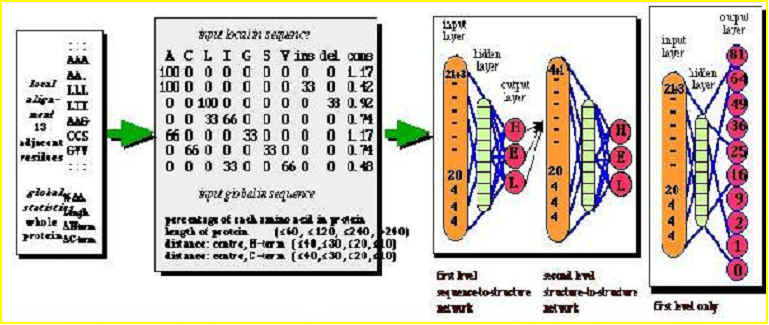
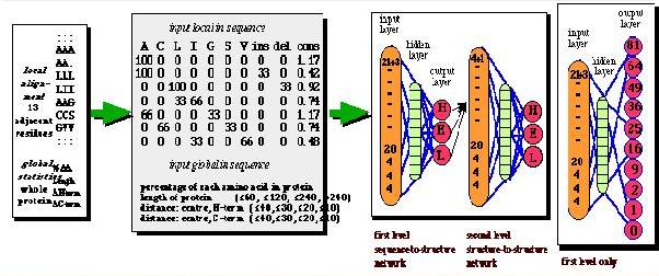
1D properties are those represented by secondary structure elements : helix (H), sheet (E) and loops;for accessibility (buried o exposed; or accesibility precentage); for hidrophobicity etc. 1D are useful to predict 3D.
AA : Residues for the sequence
OBSsec: Observed secondary structure (E: sheet, H: helice)
OBSacc: Observed accessibility(e: exposed, b: buried)
PHDsec: Predicted secondary structure
PHDacc: Predicted accessibility
Servers and programas
SECONDARY STRUCTURE PREDICTION:
Evaluation: EVA| PredictProtein
(PHDsec) |
PHDsec predicts the secondary structure multiple alignments. Neural networks (reliability = 72%, Rost & Sander, PNAS, 1993 , 90, 7558-7562; Rost & Sander, JMB, 1993 , 232, 584-599; and Rost & Sander, Proteins, 1994, 19, 55-72). | example [Output] |
| JPred | Jpred e In the case of one query: it generates an automatic alignment with clustal, which is filtered with SCANPS. | Ejemplo [Output] |
| PsiPred | PSIPRED integrates neural networks "two feed-forward" which analyses the Psi-Blast output(Altschul et al., 1997). Reliability Q3 = 77%. | Example [Output] |
Training
żWhat can you say about the secondary structure of this query?Use the urldescribed in theory section.
1. Send these sequences to secondary structure predictions servers. (PHD, JPred, PsiPred). Compare the results.
Then send it to the signal peptide... (SignalP)
- Optional: generate a multiple alignment and send it to any server acepting this input. (JPred). Compare the results with the ones obtained when a unique sequence is sent.
>1_T0112 Ketose Reductase / Sorbitol
Dehydrogenase, Bemisia argentifolii
MASDNLSAVL YKQNDLRLEQ RPIPEPKEDE VLLQMAYVGI CGSDVHYYEH GRIADFIVKD PMVIGHEASG
TVVKVGKNVK HLKKGDRVAV EPGVPCRRCQ FCKEGKYNLC PDLTFCATPP DDGNLARYYV HAADFCHKLP
DNVSLEEGAL LEPLSVGVHA CRRAGVQLGT TVLVIGAGPI GLVSVLAAKA YGAFVVCTAR SPRRLEVAKN
CGADVTLVVD PAKEEESSII ERIRSAIGDL PNVTIDCSGN EKCITIGINI TRTGGTLMLV GMGSQMVTVP
LVNACAREID IKSVFRYCND YPIALEMVAS GRCNVKQLVT HSFKLEQTVD AFEAARKKAD NTIKVMISCR QG
>APTE_DROME
MGVCTEERPVMHWQQSARFLGPGAREKSPTPPVAHQGSNQCGSAAGANNNHPLFRACSSSSCPDICDHST
>AREA_EMENI
MSGIAQLRLSDRVSNTPTTTADTVSDAMNLDDFIIPFSPSDHPSPSTTKASEATTGAIPIKARRDQSASE
>ARG1_YEAST
MTSNSDGSSTSPVEKPITGDVETNEPTKPIRRLSTPSPEQDQEGDFEEEDDDDKFSVSTSTPTPTITKTK
2. Send this sequence to TM-preodiction servers(TMHMM),
>2_636 AA
MEGPAFSKPL KDKINPWGPL IILGILIRAG VSVQHDSPHQ VFNVTWRVTN LMTGQTANVT SLLGTMTDAF
PKLYFDLCDL IGDDWDETGL GCRTPGGRKR ARTFDFYVCP GHTVPTGCGG PREGYCGKWG CETTGQAYWK
PSSSWDLISL KRGNTPRNQG PCYDSSAVSS NIKGATPGGR CNPLVLEFTD AGKKASWDGP KVWGLRLYRS
TGIDPVTRFS LTRQVLNIGP RVSIGPNPVI TDQLPPSRPV QIMLPRPPQP PPPGAASIVP ETAPPSQQPG
TGDRLLNLVD GAYRALNLTS PDKTQECWLC LVAGPPYYEG VAILGTYSNH TSAPANCSVA SQHKLTLSEV
TGQGLCVGAV PKTHQALCNT TQTSSRGSYY LVAPTGTMWA CSTGLTPCIS TTILNLTTDY CVLVELWPRV
TYHSPSYVYG LFERSNRHKR EPVSLTLALL LGGLTMGGIA AGIGTGTTAL MATQQFQQLQ AAVQDDLREV
EKSISNLEKS LTSLSEVVLQ NRRGLDLLFL KEGGLCAALK EECCFYADHT GLVRDSMAKL RERLNQRQKL
FESTQGWFEG LFNRSPWFTT LISTIMGPLI VLLMILLFGP CILNRLVQFV KDRISVVQAL VLTQQYHQLK
PIEYEP
3. Send this sequence to(NetOGly, NetPhos)
>3_41 AA
ASYDGHKLVAGYDFTPPSTPSTDDPNVCREYSYKLGTYGAP
>4_153 AA
ASQKRPSQRHGSKYLATASTMDHARHGFLPRHRDTGILDSIGRFFGGDRGAPKNMYKDSHHPARTAHYGSLPQKSHGRTQ
DENPVVHFFKNIVTPRTPPPSQGKGRKSAHKGFKGVDAQGTLSKIFKLGGRDSRSGSPKPELVISALIVESRR
| [BACK TO MAIN MENU] |